
The Precision Timing Chain: How Reference Clocks, Hardware Timestamps, and Servo Control Work Together
Modern industrial networks, 5G infrastructure, distributed data-acquisition systems, and automotive Ethernet platforms increasingly depend on a shared and dependable understanding of time. Distributed controllers must execute events in the correct sequence, measurement nodes must correlate samples accurately, and network devices must schedule traffic within tightly controlled windows.
IEEE 1588 provides the message exchange needed to compare clocks across a network, but protocol support alone does not create an accurate clock. Real synchronization performance depends on how the reference time is generated, where packet events are timestamped, how path delays are corrected, and how the local oscillator is disciplined.
A practical precision timing system therefore combines three essential layers: a stable reference source, deterministic hardware timestamp measurements, and a servo loop that converts those measurements into a controlled local clock.
IEEE 1588 support does not automatically guarantee precise synchronization.
A datasheet may list integrated PTP, hardware timestamping, nanosecond synchronization, or TSN-ready timing. However, the final result still depends on the quality and behavior of the complete timing chain.
Your achievable synchronization accuracy depends on:
The complete precision timing chain
Precision is created by the complete chain—not by a single protocol checkbox, oscillator specification, or timestamp feature.
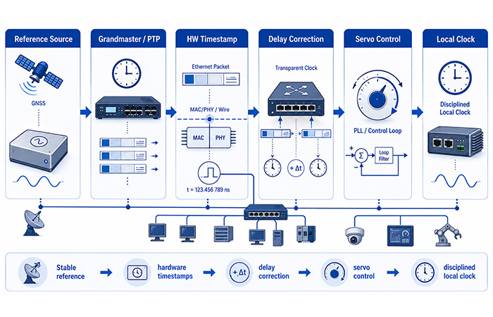
Why Precision Timing Requires a Complete System Chain
When you evaluate a precision timing system, it is easy to focus on one visible feature, such as an oscillator specification, an IEEE 1588 checkbox, or a claimed timestamp resolution. In practice, accurate synchronization depends on a complete chain in which every layer measures, transfers, or corrects a different part of time.
You can understand this chain more clearly by separating it into four engineering layers. Each layer answers a different question and owns a different part of the total timing error budget.
Time-Source Layer
This layer establishes the frequency and time basis used by the rest of the system.
Typical components
GNSS receiver, atomic frequency reference, OCXO, TCXO, rubidium oscillator, cesium reference, 1PPS, and 10 MHz reference.
Key question: Where does your time and frequency reference come from?
Network-Measurement Layer
This layer records when timing packets are transmitted and received at defined event boundaries.
Typical mechanisms
IEEE 1588 Sync, Follow_Up, Delay_Req, Delay_Resp, Pdelay messages, and hardware ingress or egress timestamps.
Key question: When did the network event actually occur?
Delay-Correction Layer
This layer identifies and corrects the delay introduced by links, switches, forwarding queues, and asymmetric paths.
Typical mechanisms
E2E, P2P, Transparent Clock, correctionField, Residence Time, and path-asymmetry compensation.
Key question: How much time did the packet spend inside the network path?
Clock-Discipline Layer
This layer converts timestamp observations into controlled phase and frequency adjustments for the local clock.
Typical mechanisms
Offset estimator, rateRatio estimator, PI servo, DPLL, PHC adjustment, DCO, NCO, and PLL control.
Key question: How does the endpoint align and maintain its local clock?
The complete precision timing chain
Each layer owns a different part of the error budget. A stable oscillator cannot compensate for an incorrectly located timestamp boundary, and precise packet timestamps cannot eliminate an unmodelled asymmetric path delay.
Where Precision Time Begins: Reference Sources and Local Oscillators
Before your network can distribute precise time, the Grandmaster must first establish a dependable frequency and phase reference. This is where two related but different requirements become important: absolute time traceability and local frequency stability.
Understanding the difference helps you choose the right combination of GNSS reception, oscillator technology, holdover capability, and clock-control hardware for your synchronization target.
Absolute Time Traceability
GNSS receivers commonly provide your system with UTC-traceable time, time-of-day information, 1PPS output, and strong long-term accuracy.
What GNSS contributes
Availability risks
Signal blockage, antenna faults, receiver noise, jamming, spoofing, and temporary loss of satellite visibility can interrupt or degrade the external reference.
Local Frequency Stability
A TCXO, OCXO, rubidium oscillator, atomic reference, clock synthesizer, or PLL maintains the local clock between network updates and during temporary loss of the external reference.
What local stability determines
- How much your clock drifts between PTP updates
- How long the system can maintain useful holdover after GNSS loss
- How aggressively the servo must correct frequency error
- How stable the clock remains across temperature changes
- How phase noise contributes to short-term time error
The reference source determines how the Grandmaster establishes and maintains its frequency and phase basis. GNSS receivers, TCXOs, OCXOs, rubidium devices, PLLs, and clock-distribution components each contribute different stability, noise, aging, and holdover characteristics. When you are evaluating the broader clock architecture, you can explore the engineering topics covered under Reference Oscillators & Timing.
Engineering distinction
GNSS commonly provides UTC-traceable time, while high-stability oscillators maintain local frequency continuity and holdover when the external reference is noisy or temporarily unavailable. They perform complementary roles rather than acting as interchangeable sources.
| Source | Main Contribution | Main Limitation |
|---|---|---|
| GNSS | UTC traceability and long-term timing accuracy | Depends on signal availability and receiver integrity |
| TCXO | Cost-effective local stability | Moderate temperature drift and holdover |
| OCXO | Improved frequency stability across temperature | Higher power, warm-up time, and cost |
| Rubidium | Strong local holdover and long-term frequency stability | Cost, size, power, and long-term aging |
| PLL / DPLL | Clock conditioning, tracking, and controlled output generation | Performance depends on reference quality and loop design |
Why Software Packet Timing Is Not Deterministic
When software records the arrival or departure of a timing packet, it usually records when the operating system or application becomes aware of that packet—not when the Ethernet frame actually crossed the network interface.
Between the physical interface and your software stack, the packet may pass through NIC receive rings, DMA transfers, interrupt handling, driver queues, multi-core scheduling, packet buffers, and application processing. Each stage introduces delay that can change with system load.
Common sources of software timestamp uncertainty
Software timestamp
When software processes the packet
The recorded time may include queueing, DMA, interrupt, scheduling, and processing delays that vary with CPU and network load.
Typical result: microsecond-scale uncertainty with load-dependent jitter and long-tail excursions.
Hardware timestamp
When the packet crosses a defined hardware boundary
The event is captured at a defined MAC, PHY, switch, or FPGA boundary before software queues and operating-system scheduling can alter the observation time.
Typical result: lower and more repeatable uncertainty, with remaining error tied to hardware resolution, pipeline placement, and calibration.
Hardware timestamping improves determinism, but it does not remove every source of error.
Hardware timestamping removes much of the non-deterministic software path, but fixed pipeline delay, timestamp quantization, clock-domain crossing, event-boundary placement, and temperature-dependent calibration still remain part of your timing error budget.
Removing software uncertainty is only the first step. You must still define where timestamp truth is created inside the hardware data path—and determine which delays remain between that capture point and the physical wire event.
How IEEE 1588 Hardware Timestamping Measures Network Events
Once you remove most of the software delay from the measurement path, the next question becomes more precise: where does your system define the actual transmit or receive event? In an IEEE 1588 timing system, synchronization accuracy depends heavily on whether timestamps are captured at a repeatable MAC, PHY, switch, or FPGA boundary.
The PTP message exchange provides four primary observations—t1, t2, t3, and t4—but those values are only useful when each timestamp represents a clearly defined event and remains consistent across traffic load, temperature, resets, and link changes.
The Four Timestamps Behind the PTP Delay Estimate
You do not need to begin with complex equations. First, make sure each timestamp corresponds to the intended ingress or egress event in the timing path.
Master Egress
The time at which the Grandmaster sends the Sync message from its defined transmit boundary.
Slave Ingress
The time at which the Slave receives that Sync message at its defined receive boundary.
Slave Egress
The time at which the Slave sends its Delay_Req message from the transmit boundary.
Master Ingress
The time at which the Grandmaster receives the Delay_Req message at its receive boundary.
The value of t1–t4 depends less on the labels themselves and more on whether all four timestamps are created at deterministic, consistent, and correctly calibrated hardware boundaries.
Comparing MAC, PHY, Switch, and FPGA Timestamp Boundaries
Moving the timestamp closer to the physical wire event generally reduces software and internal pipeline uncertainty. However, it also increases the responsibility for fixed-delay calibration, asymmetry control, temperature characterization, and coherent timestamp readout.
MAC Timestamping
Common SoC / NIC ChoiceMAC-based timestamping is widely used because it is usually well integrated with drivers, network stacks, and a PTP Hardware Clock.
Strengths
- Mature integration
- Good driver support
- Straightforward PHC connection
- Suitable for many industrial endpoints
Risks to Verify
- Unclear MAC pipeline location
- Queueing after timestamp capture
- Clock-domain crossing
- Multi-queue packet association
PHY Timestamping
Closest to the WirePHY timestamping captures the packet event closer to the Ethernet signal boundary, reducing uncertainty from MAC pipelines, queues, and software handling.
Strengths
- Closer to the wire event
- Lower MAC pipeline uncertainty
- Reduced software-path influence
- Well suited to high-accuracy systems
Risks to Verify
- Fixed internal delay
- Temperature-dependent drift
- Link asymmetry
- PHY-to-host readout coherency
- Greater calibration burden
The critical design question is therefore not simply whether a platform supports PTP, but where the timestamp is captured and which delays remain between that point and the physical wire event. A detailed guide to IEEE 1588/PTP Hardware Timestamping examines PHY, MAC, switch, and FPGA capture boundaries, together with the calibration, ordering, and verification responsibilities associated with each implementation.
Switch Timestamping
Multi-Hop CorrectionA PTP-aware switch can capture ingress and egress events, measure Residence Time, and update the correctionField as packets move through the network.
Strengths
- Measures Residence Time
- Supports Transparent Clock operation
- Improves multi-hop delay ownership
- Useful in TSN and telecom networks
Risks to Verify
- Inconsistent switch capabilities
- Queue-dependent delay not fully measured
- Unclear correction ownership
- Mixed PTP-aware and non-aware paths
FPGA Timestamping
Maximum Design ControlFPGA implementations let you define the event boundary, counter architecture, packet association, and calibration logic for specialized measurement or synchronization systems.
Strengths
- Custom event boundaries
- Highly deterministic pipelines
- Custom packet association
- Suitable for specialist systems
Risks to Verify
- Reference clock quality
- Timestamp counter design
- Clock-domain crossing
- Reset and retraining calibration
- Packet-to-timestamp association
Boundary trade-off
One-Step and Two-Step Timestamp Delivery
One-Step and Two-Step PTP are sometimes presented as if one method were automatically more accurate or more advanced. In reality, each method places responsibility in a different part of the transmit and timestamp-delivery path.
Your choice should be based on where the precise t1 timestamp is created, how it reaches the receiver, and whether the complete path remains correct under traffic load, queueing, packet loss, and reordering.
In-frame timestamp insertion
One-Step PTP
In a One-Step implementation, the precise t1 value is inserted directly into the Sync frame as that frame moves through the egress path.
What the hardware must guarantee
- The t1 timestamp is captured at the intended egress boundary
- The frame can be modified without corrupting FCS or checksum handling
- No unaccounted queueing remains after timestamp insertion
- Traffic shaping does not move the real wire event away from the timestamp point
Typical Failure Signatures
- Stable but incorrect offset bias
- Offset changes when traffic load changes
- Timestamp no longer represents the wire event after shaping or queueing
Sync and Follow_Up delivery
Two-Step PTP
In a Two-Step implementation, the Sync frame is transmitted first. A separate Follow_Up message then carries the precise t1 timestamp created by the egress hardware.
What the system must guarantee
- Every Sync frame is paired with the correct Follow_Up
- sequenceId and portIdentity remain consistent
- Follow_Up latency remains bounded and observable
- Packet loss or reordering does not corrupt timestamp association
Typical Failure Signatures
- Delayed Follow_Up messages
- Lost or incorrectly paired timestamps
- Packet reordering
- Periodic offset jumps while the Ethernet link still appears normal
How to Choose Between One-Step and Two-Step
Choose One-Step when:
Your platform provides proven in-frame timestamp insertion at the true egress boundary and you control the complete transmit pipeline.
Choose Two-Step when:
Separating timestamp creation from frame transmission simplifies the hardware path and your implementation can guarantee reliable Follow_Up association.
One-Step reduces dependence on a second timing message but increases frame-modification and pipeline-placement responsibility. Two-Step simplifies the transmit packet path but requires reliable timestamp delivery, ordering, and association. In both cases, the timestamp path must be treated as part of the complete timing loop.
How Switches Correct Residence Time and Network Delay
Accurate endpoint timestamps are only one part of a complete IEEE 1588 timing path. Once a timing packet begins moving through switches, queues, and physical links, additional delay terms are introduced that neither endpoint can observe directly.
To keep those delays from appearing as unexplained timing noise, each device in the path must measure and report the terms it can observe at its own defined hardware boundaries.
Residence Time Is Not a Fixed Constant
Residence Time is the time between a packet entering and leaving a forwarding device at defined ingress and egress timestamp boundaries.
In a real network, this delay may change from packet to packet. A switch can process the same PTP message differently depending on its queue state, traffic class, port activity, and internal forwarding architecture.
Factors that can change switch residence time
What a Transparent Clock Contributes
A Transparent Clock measures residence time between defined hardware boundaries. It does not make network delay disappear. Instead, it makes a delay term visible so the endpoint can include that term in its timing calculation.
Capture Ingress Time
Record when the PTP packet enters the forwarding device at the selected hardware boundary.
Measure Residence Time
Calculate the time between the selected ingress and egress timestamp boundaries.
Update correctionField
Add the measurable delay contribution so downstream devices can account for it explicitly.
Forward the Packet
Send the packet onward with its measured switch delay represented in the correction chain.
E2E and P2P Solve Different Network Problems
IEEE 1588 can estimate path delay end to end or measure delay between neighboring devices. The right mechanism depends on your network depth, traffic behavior, and ability to make each delay contribution observable.
End-to-End Delay Measurement
E2EIn an E2E implementation, the endpoint uses t1, t2, t3, and t4 to estimate the mean delay across the complete path between Master and Slave.
Usually suitable when:
- The network path is relatively simple
- Only a small number of intermediate devices are present
- Residence-time variation is controlled
- Cross traffic remains within the timing budget
Peer-to-Peer Delay Measurement
P2PIn a P2P implementation, each timing-aware device measures the Neighbor Delay to the device directly connected to it.
Usually suitable when:
- The timing path contains multiple switches
- The system uses TSN or 802.1AS/gPTP
- Traffic load creates measurable PDV
- You need to isolate an abnormal link or device
Correction ownership
Let Each Component Own the Delay It Can Measure
| Component | Timing Responsibility |
|---|---|
| Endpoint | Correct t1–t4 capture, timestamp ordering, packet association, and Sync/Follow_Up pairing. |
| Transparent Clock | Residence Time measurement and correctionField accumulation across the forwarding path. |
| PHY / Calibration Layer | Fixed pipeline delay, link asymmetry, media-dependent offsets, and temperature-sensitive calibration terms. |
| Servo | Residual offset tracking, measurement filtering, frequency correction, and dynamic recovery. |
The component that can observe a delay term at the correct physical boundary should own that term. If ownership is unclear, the delay may reappear as load-dependent or temperature-dependent timing error that the endpoint cannot explain or correct reliably.
How the Servo Disciplines the Local Clock
A timestamp is a measurement, not a clock. After your system captures packet events and estimates path delay, it still needs a control loop that converts those observations into practical phase and frequency adjustments.
The PTP servo compares the local timebase with the Master, filters measurement noise, estimates oscillator behavior, and then adjusts the local clock without introducing unnecessary phase steps or instability.
What the Servo Receives
Offset
The estimated time difference between your local clock and the Grandmaster at the selected event boundary.
Path Delay
The network delay estimate used to separate clock offset from packet travel time.
May include E2E or P2P measurements, correctionField values, Residence Time, and calibrated link terms.
rateRatio
The estimated frequency difference between the local oscillator and the Master, used to control long-term drift.
What the Servo Can Control
The control output depends on your platform. The servo may adjust a digital clock register, change an oscillator control word, or drive a dedicated timing component.
This is why the complete function should be described as servo control and local clock discipline, rather than simply calling every implementation a PLL.
Loop Bandwidth Controls the Main Trade-Off
Servo bandwidth determines how quickly your clock follows legitimate timing changes and how strongly it reacts to packet-delay variation or timestamp noise.
Wider Loop Bandwidth
Faster ResponseBenefits
- Faster initial lock
- Faster recovery after a path change
- Better tracking of oscillator temperature drift
Risks
- Follows Packet Delay Variation
- Follows timestamp measurement noise
- Produces a noisier local time output
Narrower Loop Bandwidth
Smoother OutputBenefits
- Smoother local time output
- Lower short-term noise
- Less sensitivity to transient PDV
Risks
- Longer lock time
- Slow recovery after path changes
- Weak tracking of oscillator drift
- Residual offset may remain for longer
Where timestamps and oscillators meet
Better hardware timestamps lower the measurement noise floor, giving the servo more freedom to balance settling time, oscillator tracking, and short-term stability. This is where your reference oscillator, packet-event measurements, and control loop become one complete precision timing system.
Why Timing Systems Pass on the Bench but Fail in the Field
A precision timing design can look stable during a controlled laboratory test and still produce offset jumps, drift, or long-tail errors after deployment. The difference is usually not that IEEE 1588 suddenly stops working. The field introduces traffic, temperature, path, and recovery conditions that the original test did not reproduce.
To understand a failure, you should look for correlation. If the timing error changes with network load, cable replacement, temperature, or link retraining, that pattern often points directly to the layer that owns the problem.
Traffic Load Changes the Delay Distribution
A bench test may contain only low-rate PTP traffic, while the deployed network must handle application data, control traffic, video streams, and background communication.
As traffic increases, cross traffic, queue growth, QoS scheduling, port congestion, and packet buffering can widen the Packet Delay Variation seen by the timing loop.
Failure signature
Offset RMS, P99, or P99.9 becomes worse as network load increases. This often points to variable Residence Time, hidden queueing, or a servo that follows too much network noise.
Path Asymmetry Creates a Fixed Timing Bias
PTP delay calculations commonly assume that forward and reverse delays are sufficiently similar. When those directions are not equal, part of the difference appears as clock offset.
Path asymmetry can be introduced by different PHY paths, media converters, cable replacements, optical modules, switch-port pipelines, route changes, or different line-encoding paths.
Failure signature
Replacing a cable, module, PHY, or switch produces an immediate and repeatable offset step while packet rate and synchronization state still appear normal.
Temperature Changes More Than the Oscillator
Temperature affects the local frequency source, but it can also change delays inside the PHY, PLL, cable, and calibrated timing path.
A design that is calibrated at room temperature may accumulate error when oscillator frequency, PHY pipeline delay, PLL behavior, cable delay, or fixed compensation values change across the operating range.
Failure signature
Offset moves gradually with temperature even though network traffic, message rate, and topology remain unchanged.
Reset and Link Retraining Can Change the Baseline
A system may pass steady-state testing but fail to return to the same timing baseline after a reboot, link flap, or PHY retraining event.
After reset, internal pipeline latency may change, timestamp queues may be reinitialized, calibration may not be restored, or an FPGA fixed-delay baseline may no longer match the value used before the event.
Failure signature
Each reconnect, retraining event, or power cycle produces a different fixed offset even though the physical topology has not changed.
Read the correlation
Match the Failure Pattern to the Likely Error Source
| Observed Pattern | Likely Area to Investigate |
|---|---|
| Error increases with traffic load | Residence Time, queueing, PDV, or servo bandwidth |
| Offset steps after component replacement | Path asymmetry or fixed link-delay compensation |
| Offset drifts with temperature | Oscillator drift, PHY delay, PLL behavior, or calibration slope |
| Offset changes after link retraining | Pipeline state, fixed-delay calibration, queue initialization, or timestamp association |
How to Validate a Precision Timing System
A claim such as “nanosecond-level synchronization” is only useful when you know where the measurement was taken, under which network conditions, for how long, and which statistical metric was used.
Your validation plan should turn a general timing claim into a repeatable set of boundaries, test conditions, metrics, disturbances, and pass criteria. This makes results comparable across devices, firmware versions, and network topologies.
Define the Measurement Boundary
Before comparing timing results, identify exactly where local time is being compared with Master time.
A result measured at the physical wire event includes a different set of delays than a result measured inside the PHY, MAC, PHC, or application layer.
Results from different boundaries should not be compared as if they measure the same error. Always record the boundary in the test report.
Define the Statistical Metrics
A single maximum value does not tell you whether the system is normally stable or frequently produces long-tail errors.
Combine steady-state metrics with percentile and dynamic-response measurements. Offset RMS describes typical locked behavior, while P99 and P99.9 reveal excursions that averages can hide.
If you report a maximum or peak-to-peak value, include the observation window, traffic condition, topology, temperature, and packet-loss condition. Without those details, the number is not reproducible.
Define the Dynamic Test Conditions
Steady-state performance is not enough. Your system must also recover predictably when the network, clock source, or hardware state changes.
Include controlled disturbances that reproduce the conditions most likely to expose timestamp loss, path changes, calibration errors, and servo-recovery problems.
Load and Traffic
Load sweep, cross traffic, congestion, packet loss, and queue-depth changes.
Environment
Temperature sweep, warm-up, supply variation, and long-duration operation.
Topology and Path
Master switch, topology change, cable replacement, and module replacement.
Reset and Recovery
Power cycle, link down/up, PHY retraining, and firmware restart.
Timestamp Delivery
Follow_Up delay injection, packet reorder, timestamp loss, and queue stress.
Define Measurable Pass Criteria
Each requirement should produce an observable result that can be accepted or rejected without subjective interpretation.
Example pass-criteria templates
Do not apply the same 10 ns, 50 ns, or 100 ns target to every system. The correct threshold must come from your system-level timing error budget, application requirements, topology, oscillator quality, and operating environment.
A comparable timing claim
When all five elements are documented, your timing result becomes reproducible, comparable, and useful for component selection, regression testing, and field troubleshooting.
Applications That Depend on the Complete Timing Chain
A complete precision timing chain becomes valuable whenever distributed devices must share time with predictable accuracy, continuity, and recovery behavior. The requirement may appear as a nanosecond target, a scheduled traffic window, a synchronized sample, or a phase-continuity limit, but the engineering foundation remains the same.
In each application, you should evaluate the full path from the reference oscillator and Grandmaster clock to the ingress and egress timestamps, network-delay corrections, clock servo, and disciplined local clock.
Industrial TSN and Deterministic Automation
Motion controllers, robots, drives, sensors, and distributed I/O devices need a stable common timebase so actions occur in the intended sequence.
In an Industrial Ethernet or TSN network, average synchronization accuracy is not enough. Scheduled traffic, motion coordination, and deterministic execution depend on the clock remaining stable across every cycle, path, and topology change.
Your validation should focus on synchronization continuity, scheduled-window stability, path recovery, and the behavior of every Boundary Clock or Transparent Clock in the timing path.
5G and Telecom Backhaul
Telecom timing paths often cross multiple switches, transport segments, and timing-aware devices before reaching the endpoint.
In a 5G backhaul network, delay ownership becomes critical. P2P measurements, Transparent Clock operation, Packet Delay Variation, Grandmaster traceability, and oscillator holdover must work together across the complete route.
As the number of switches increases, every unmeasured residence term or correction mismatch can accumulate into a larger endpoint error.
Distributed Measurement and Data Acquisition
Distributed instruments must assign comparable time to samples and events collected at different physical locations.
For distributed data acquisition, repeatability is often more valuable than a single best-case peak result. Cross-node sample alignment, event correlation, PPS or trigger outputs, and temperature stability should be evaluated using RMS and percentile metrics over a defined observation window.
A repeatable time-error distribution gives you more confidence in measurement correlation than an isolated minimum or maximum value.
Automotive Ethernet and Zonal Architectures
Vehicle networks increasingly depend on synchronized sensing, zonal communication, scheduled traffic, and fault-aware timing distribution.
In Automotive Ethernet, synchronization must remain observable as well as accurate. Sensor fusion, scheduled communication, and zonal control require link-state monitoring, fault alarms, path-change detection, and temperature correlation.
A useful automotive timing design should let you detect, isolate, and recover from synchronization faults rather than only report a nominal accuracy target.
Broadcast and Professional AV
Audio, video, and production systems depend on low wander, stable phase, and predictable timestamp delivery.
In broadcast synchronization, periodic phase jumps may be more disruptive than a small steady offset. Follow_Up stability, PHC support, timestamp queue behavior, low wander, and smooth recovery should therefore be treated as primary selection criteria.
Engineering Checklist for Device and Network Selection
When you select a PHY, MAC, switch, NIC, FPGA platform, oscillator, or timing IC, avoid treating each component as an isolated datasheet decision. Your final result depends on how every device participates in the complete IEEE 1588 timing chain.
Use the following questions to turn broad feature claims into measurable requirements before you commit to a device or network architecture.
Reference Source and Oscillator
Timestamp Hardware
PTP Behavior and Message Handling
Network Devices and Delay Ownership
Servo and Local Clock Discipline
Final qualification
Verification Questions
Precision Timing Is a Chain, Not a Single Feature
Precision timing is not created by a single protocol feature or hardware block. The reference source establishes the frequency and phase foundation, hardware timestamps define when network events occur, delay mechanisms account for what happens across the path, and the servo converts those observations into a disciplined local clock.
A weakness at any point in this chain can limit the complete system. Stable oscillators cannot correct an incorrectly defined timestamp boundary, while accurate timestamps cannot remove unmeasured path asymmetry or poorly tuned servo behavior. Reliable synchronization therefore depends on clear ownership, measurable error terms, and validation under realistic load, temperature, topology, reset, and recovery conditions.
Frequently Asked Questions About Precision Timing
These answers clarify how reference oscillators, hardware timestamps, network-delay measurements, and clock servos work together in an IEEE 1588 synchronization system.
What is the role of a reference oscillator in IEEE 1588? +
A reference oscillator provides the local frequency basis used by the Grandmaster or Slave clock. Its stability affects how much the clock drifts between PTP updates, how accurately the servo can track the Master, and how long the system can maintain useful holdover when GNSS or another external reference becomes unavailable.
Why is hardware timestamping more accurate than software timestamping? +
Hardware timestamping records a packet event at a defined MAC, PHY, switch, or FPGA boundary. This removes much of the uncertainty caused by operating-system scheduling, interrupts, DMA batching, driver queues, and application processing. Hardware timestamps are more repeatable, although timestamp resolution, fixed pipeline delay, clock-domain crossing, and calibration still remain part of the error budget.
Is PHY timestamping always better than MAC timestamping? +
Not always. PHY timestamping is normally closer to the physical wire event and can reduce uncertainty from the MAC pipeline and software path. However, it may require stricter fixed-delay calibration, temperature characterization, asymmetry compensation, and coherent PHY-to-host readout. MAC timestamping may be a better choice when its capture boundary is clearly defined and its accuracy meets your system budget.
What is the difference between One-Step and Two-Step PTP? +
In One-Step PTP, the precise transmit timestamp is inserted directly into the Sync message as it moves through the egress path. In Two-Step PTP, the Sync message is sent first and a later Follow_Up message carries the precise transmit timestamp. Two-Step operation therefore depends on reliable pairing through sequenceId and port identity, while One-Step requires correct in-frame insertion at the intended egress boundary.
How does a PTP servo adjust the local clock? +
A PTP servo uses the estimated clock offset, network path delay, and rateRatio to determine how the local timebase differs from the Master. It can then adjust a PHC rate, DCO, NCO, DPLL, PLL, fractional divider, clock synthesizer, or FPGA counter so the local phase and frequency gradually align with the Master without introducing unnecessary jumps or instability.
Why can a PTP system work in the lab but fail in the field? +
Laboratory tests often use low traffic, stable temperature, fixed media, and an unchanged topology. Field conditions introduce Packet Delay Variation, queue growth, path asymmetry, temperature drift, module replacement, link retraining, and reset events. These conditions can expose Residence Time, calibration, timestamp-association, and servo-recovery problems that were not visible during a static bench test.