
EMI Mitigation & Spread Spectrum — Sources, Paths, and Fix Loops
This page shows fast, low-cost ways to bring power-converter EMI under control: identify where noise is generated, how it couples, and what to change first. We focus on practical levers—loop geometry, damping, input/output filtering, and spread-spectrum trade-offs—plus a repeatable measure → hypothesis → action → verify loop. Deep loop-compensation, minimum on-time, valley/peak current details are covered on sibling pages (Synchronous Buck / Boost & Buck-Boost / Layout & Snubbers / PMBus-PSM).
EMI Basics — Sources · Paths · Victims
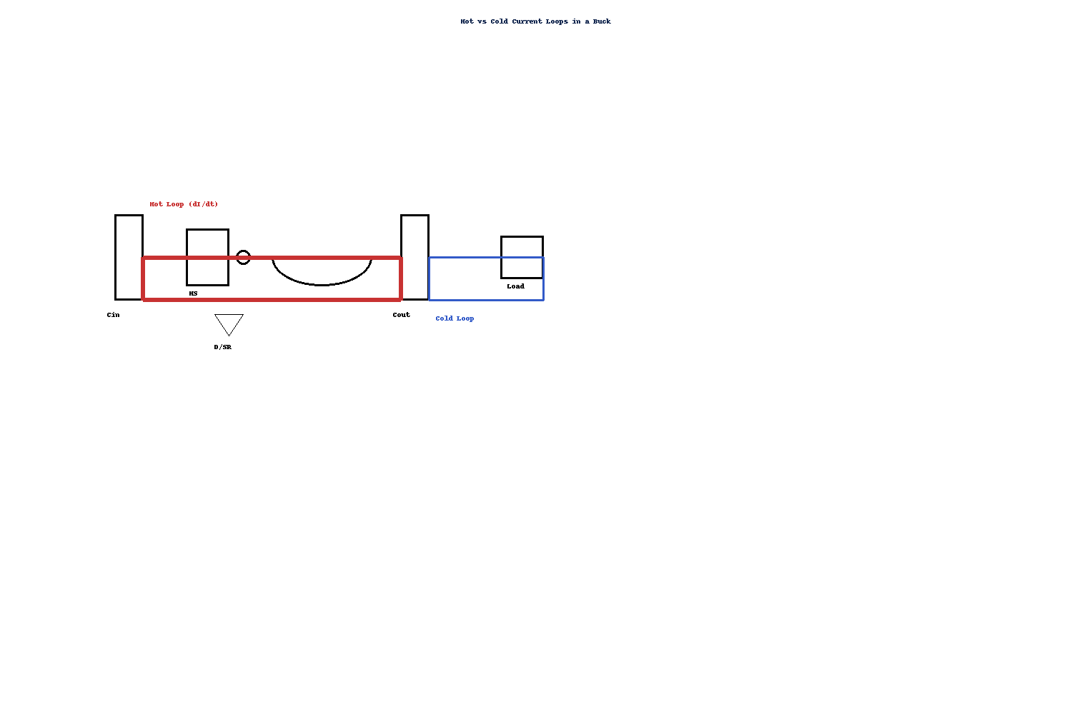
Sources. Fast edges (high dV/dt and dI/dt) excite parasitic L/C and create narrowband peaks and ringing. The hot-loop area and impedance largely set the raw amplitude and radiation efficiency—shrink the loop first, then consider filters and spread-spectrum. Expect a line spectrum around the switching frequency with sidebands from ringing and load modulation.
Paths & victims. Three dominant couplings: DM (conducted differential) through the rail/return loop and LISN path, CM (common-mode) via stray capacitances, shields and harness (the whole cable “rides” the noise), and radiated from large loop areas, slots, and cable antennas. Always classify the path first; different tools solve different paths (DM→LC/π+damping; CM→choke/shield termination; radiated→loop geometry & seams).
- Shrink the hot loop (HS FET → diode/SR → Cin) and keep the return tight.
- Keep SW copper compact; avoid routing under sensitive analog nodes.
- Fingerprint the dominant path (near-field probe / current clamp) before adding parts.
- Fix geometry & damping first; use spread-spectrum as a finishing lever.
- Log before/after spectra with identical setups to avoid “peak whack-a-mole”.
| Path | Symptoms | First Levers | Verify |
|---|---|---|---|
| DM (Conducted) | Peaks at fsw and harmonics on LISN; ripple interaction | LC/π + damping (ESR/series-R/RC); snubber | Before/after LISN overlays; Bode after heavy filtering |
| CM (Common-mode) | Cable/housing currents; radiated fails despite DM fixes | CM choke; 360° shield termination; edge-rate control | Clamp current on harness; chamber/antenna near-field scan |
| Radiated | Peaks vs loop geometry; enclosure seams and slot resonances | Shrink hot loop; stitch returns; fix seam impedance; shorten cables | Near-field probe maps; A/B on cable routing and seam bonding |
With the path classified, move to Measurement: keep cables repeatable, run a quick LISN pre-scan and near-field sweep to pick the right lever before investing in parts.
Measurement & Limits — Quick, Repeatable, Honest
Conducted (150 kHz–30 MHz): LISN · Cable Discipline · Termination Consistency
For conducted pre-scans, verify LISN bonding, fix cable length and routing across runs, and keep a consistent ground/termination topology. Start with a wide sweep to reveal peaks, then re-scan around hot spots. Log both Peak and Average detectors under identical operating points.
Radiated: Near-Field Probes · Current Clamp · Reproducible Posture
Use near-field H/E probes around the SW node, inductor, and harness to fingerprint sources. Place a current clamp on the cable to expose common-mode components. Photograph the setup (distances, cable paths, antenna/probe posture) so every fix is re-measured in the same geometry.
| Domain | Focus | Tools | Reproducibility |
|---|---|---|---|
| Conducted (150 kHz–30 MHz) | Peaks at fsw & harmonics on LISN; ripple interaction | LISN, spectrum analyzer (Peak/Avg), stable mains impedance | Lock cable length/route; repeat operating points & terminations |
| Radiated | Hot spots near SW node, inductor, seams; harness as antenna | Near-field H/E probes, current clamp on harness, chamber/antenna checks | Photograph layout & posture; annotate distances for exact A/B overlays |
Pre-scan steps (fast loop)
- Fix cable length & route; confirm LISN ground/bonding.
- Record operating points (VIN, load, modes) and keep constant across runs.
- Wide sweep → identify top-N peaks; then zoom around each bucket.
- Capture Peak & Average traces; export raw files with timestamps.
- Near-field & clamp fingerprint (DM vs CM) to choose the right lever.
- Photograph the setup; save into the same run folder as spectra.
Helpful resources: EMI Pre-Compliance Checklist (PDF), Spread-Spectrum Playbook (PDF).
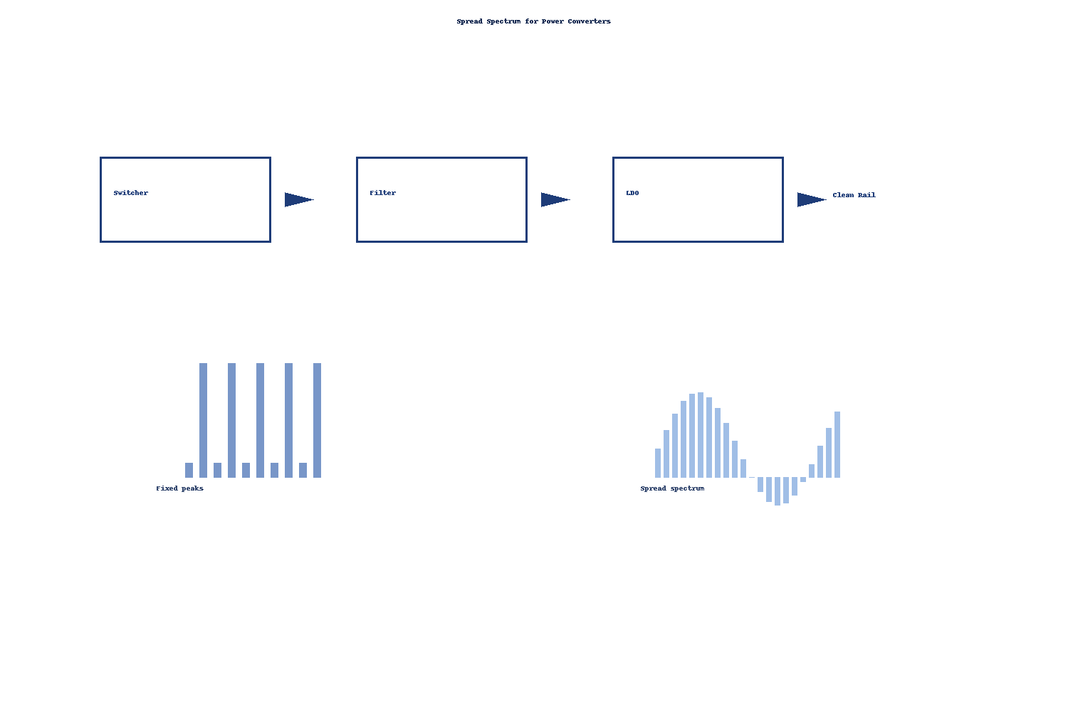
Spread Spectrum — Profiles, Trade-offs, and Verification
Profiles & selection logic
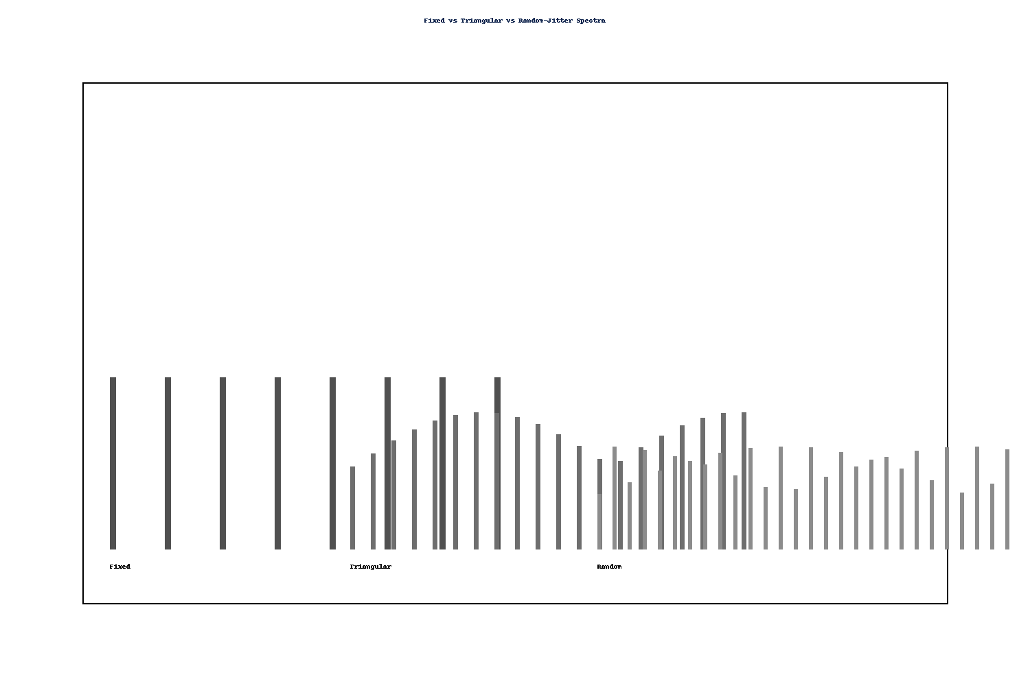
Choose between Triangular sweep and Random jitter, and decide center-spread vs down-spread. For tight timing/sync domains, down-spread is often safer; for RF-sensitive products, random jitter tends to reduce discrete tones, while triangular is easier to model and reproduce.
Side-effects checklist
- Audible noise & beat tones with other clocks or load cycles.
- Loop-gain variation near crossover; ripple redistribution & efficiency shifts.
- Energy relocation into sensitive bands (AM/FM/ISM/automotive); conducted vs radiated can diverge.
| Type / Bias | Strengths | Risks | Best-fit scenarios | Notes |
|---|---|---|---|---|
| Triangular sweep | Predictable skirts; easy to tune & reproduce | Discrete skirts may land on RF masks | Systems that favor modeling/validation repeatability | Sweep rate: avoid audible; confirm with LISN overlay |
| Random jitter | Lower discrete tones; often quieter for radios | Harder to analyze; repeatability depends on RNG | RF-sensitive products; coexistence with wireless | Seed & bounds must be documented in production |
| Center-spread | Average fsw unchanged; minimal timing drift | Risk of pushing energy to both sides of masks | Tight regulation loops; synced PWM domains | Verify loop gain around crossover |
| Down-spread | Safer for timing budgets; avoids exceeding max fsw | Lower average fsw may affect ripple & efficiency | Timing-critical / multi-domain sync systems | Check ripple change & audible interaction |
Verification flow
- Capture baseline conducted & radiated spectra at fixed operating points.
- Enable profile A/B; sweep depth and modulation rate.
- Select the minimum effective depth that meets limits with margin.
- Re-check loop stability, ripple, efficiency, and cross-domain timing/audio.
See also: Spread-Spectrum Playbook (PDF), RC Snubber Quick Rules (PDF).
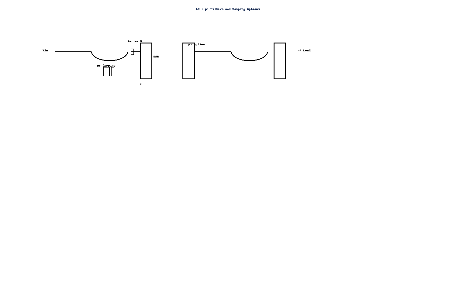
Input/Output Filtering — LC/π Selection & Damping
LC/π selection: target corner & controlled damping
Pick L and C from the desired corner frequency and ripple goals, then add loss on purpose to avoid peaking: via capacitor ESR, a series resistor, or an RC damper across L/C. π filters provide steeper DM attenuation but may introduce a mid-node resonance— verify interactions with the control loop.
Damping strategies (from light to heavy)
| Method | Mechanism | Strengths | Trade-offs | Use when… | Verify |
|---|---|---|---|---|---|
| Cap ESR | Intrinsic loss flattens the LC peak | No extra parts; simple | ESR varies with temp/age; limited range | Mild peaking; cost/space constrained | Ripple, temperature drift, LISN overlay |
| Series-R | Adds controlled DM loss in series path | Predictable damping; scalable | Efficiency drop; power rating needed | Moderate peaking; tunable attenuation | Thermals, step load transient, Bode |
| RC across L | Bypasses HF energy and damps the L branch | Strong peak control; localizes loss at HF | Power in R; layout proximity matters | Sharp peaking near LC corner; ringing | Scope overshoot; resistor heating |
| RC across C | Adds HF shunt loss at the cap legs | Simple routing; broad HF damping | May raise ripple; part tolerance sensitive | Distributed HF hash; broad skirts | Ripple spectrum; LISN & scope decay |
When to use a CM choke (cable egress & shields)
If common-mode dominates (harness currents, radiated fails despite DM fixes), place a CM choke near the cable egress and implement 360° shield termination. CM chokes do little for DM peaking; pair them with geometry fixes and damping.
If peaking is driven by SW-node ringing, move to Snubbers. For CM-dominated fixes, see “Shielding & Cables”.
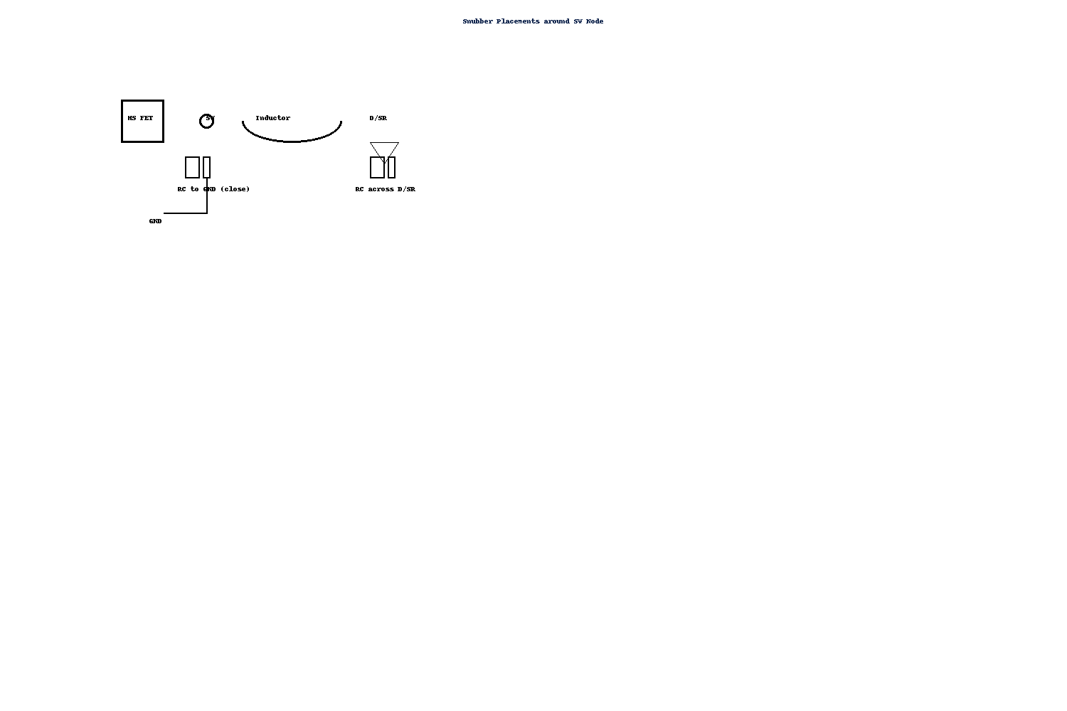
Snubbers — Fast Sizing, Placement, and Scope Verification
Types & placement
Use RC to ground at the SW node, RC across the diode/synchronous MOSFET, or an RC-R variant for stronger damping. Keep loops short, place parts physically close to the node, and return to a quiet ground.
Quick sizing & scope method
- Measure ringing frequency fr and estimate node capacitance Cnode.
- Estimate L ≈ 1 / ( (2π·fr)² · Cnode ).
- Start Csnub ≈ 0.5–1.0 × Cnode.
- Pick R ≈ √( L / Csnub ); begin slightly overdamped, then trim.
- On the scope, minimize overshoot and ringing without excessive power loss.
| Symptom | Likely cause | Quick action | Verify |
|---|---|---|---|
| Resistor overheating | Over-damping or too small package/power rating | Reduce C or increase R; choose higher-power package | Thermal rise at worst-case duty/load |
| Overshoot persists | Under-damping; parasitic L in placement | Increase C slightly; move parts closer to SW node | Scope overshoot/settling vs baseline |
| New peak appears | Alternate resonance excited by values/placement | Sweep R in small steps; fine-trim C | LISN overlay / near-field map after change |
| CM noise increases | Snubber return creates CM path; geometry too large | Shorten return; review ground reference; consider CM choke | Clamp current on harness; radiated pre-scan |
Detailed sizing steps: RC Snubber Quick Rules (PDF).
Layout Levers — Minimal Checklist That Moves the Needle
Core principles
- Shrink the hot loop: HS FET → diode/SR → Cin → return. Keep the physical triangle compact.
- SW copper compact: do not route under sensitive analog nodes; define a keepout if needed.
- Rsense / analog star-ground: separate high-dI/dt returns; Kelvin sense only to the sense element.
- Place DM/CM filters at the cable egress: control the path at the boundary first.
Return paths & reference planes
Maintain a continuous reference plane. Put HF bypass caps close to the switch and return via short, low-inductance vias. Avoid slots under fast return paths. Prefer multilayer stacks: parts on top, solid inner-layer ground, short and direct traces.
Minimal actionable checklist
- Draw the hot-loop outline; make it visibly shorter/tighter after each placement tweak.
- Keep SW node local; fence it from analog/Kelvin sense routes.
- Place Cin HF cap so HS/LS/source pins and cap pads form a tight triangle.
- Star the analog ground; single-point return to power ground after Rsense/Kelvin.
- Put CM/DM filters next to the connector; route cables consistently.
Deep layout patterns, scope shots, and snubber placement live on the sibling page: Layout & Snubbers.
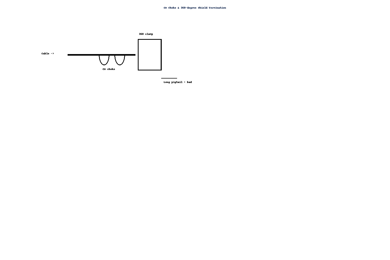
Shielding & Cables — Control the Common-Mode Path
360° shield termination beats long pigtails
Use a 360° clamp or full-wrap termination for the cable shield at the chassis. Keep the bond short, wide, and circumferential to lower HF impedance. Long pigtails add inductance and undo shielding at high frequency—avoid them wherever possible.
Seams and conductive finishes
Lower seam impedance with frequent fasteners and wide, clean contact. Break anodize/paint where electrical bonding is required: use conductive gaskets, finger-stock, plating, or localized mask-offs. Slot geometry and poor contact increase radiated peaks.
Cables and CM choke placement
If common-mode dominates, put a CM choke near the cable egress on the shield side. Keep cables short and routed over a reference plane or the chassis. Where appropriate, evaluate single-ended shield termination vs multi-point schemes with pre-scans.
| Item | Do | Don’t | Verify |
|---|---|---|---|
| Shield termination | 360° clamp; short, wide bond to chassis | Long pigtail ground leads | Radiated pre-scan; clamp current on harness |
| Seams & coatings | Break paint/anodize where bonding is needed; use gaskets | Rely on cosmetic contact through coatings | A/B with near-field probe along seam |
| CM choke placement | Place near egress; pair with 360° shield clamp | Place far from connector or before long cable runs | Clamp current drop; chamber scan delta |
| Cable length & routing | Keep short and repeatable; route over ground/chassis planes | Floating in air; inconsistent lengths and loops | Photographic record of posture; repeatability across runs |
Next: close the loop with a repeatable Fix-Loop Playbook, or revisit Measurement to ensure posture consistency.
Fix-Loop Playbook — Fingerprint → Classify → Change One → Verify
- Fingerprint: run LISN pre-scan (150 kHz–30 MHz), near-field map around SW node/inductor, and a current-clamp on the harness. Log top-N peaks.
- Classify: assign each peak to DM, CM, or radiated. Map levers: DM→LC/π + damping; CM→choke & 360° shield; radiated→geometry/seams.
- Change one variable: add one lever at a time (e.g., RC snubber, series-R, CM choke, down-spread). Keep operating points and posture identical.
- Verify & record: overlay before/after spectra (Peak/Avg), photograph posture, document settings and side-effects. Aim for a 3–6 dBµV margin.
Remediation log template
| Change | Path (DM/CM/Rad) | Domain | Before | After | Δ | Notes / Side-effects |
|---|---|---|---|---|---|---|
| Add RC snubber @SW→GND | DM | Conducted | 123 kHz @ 66 dBµV (Peak) | 123 kHz @ 58 dBµV (Peak) | −8 dBµV | Ripple +2 mVpp; R hot @50°C |
| Add CM choke @egress | CM | Radiated | 40–60 MHz peak over limit | Within limit +4 dB margin | pass | Clamp current −60% |
Templates & procedures: EMI Pre-Compliance Checklist (PDF), RC Snubber Quick Rules (PDF), Spread-Spectrum Playbook (PDF).
Vendor Options — Spread-Spectrum Capabilities (TI · ST · NXP · Renesas · onsemi · Microchip · Melexis)
Spread spectrum reduces peak amplitude by redistributing energy; it does not remove energy. Profiles (Triangular / Random) and bias (Center / Down) have different system impacts. The table below is a series-level overview—always verify the latest datasheet for exact capabilities.
| Vendor | Product type | Spread spectrum | Depth / Rate (e.g.) | Notes | Docs |
|---|---|---|---|---|---|
| TI | Buck controllers / PMIC | Triangular / Random; Center/Down (model-dependent) | e.g., 3–10% depth; kHz-range sweep | Sync options, phase interleaving on some families | Datasheet |
| ST | Buck / Module | Triangular; often Down | e.g., 3–8%; audio-safe rates | Automotive-grade options available | Datasheet |
| NXP | PMIC / Automotive | Random / Triangular (series-specific) | e.g., 3–6%; randomized rates | Focus on car-grade coexistence | Datasheet |
| Renesas | Controllers / PMIC | Triangular / Random; Center/Down | e.g., 3–10%; vendor-defined ranges | Sync & frequency foldback notes | Datasheet |
| onsemi | Controllers / Modules | Triangular; often Down for timing safety | e.g., 4–8%; kHz sweep | Automotive & industrial lines | Datasheet |
| Microchip | Controllers / PMIC | Random / Triangular (device-specific) | e.g., 3–6%; audio-aware dithering | Good docs for spread configuration | Datasheet |
| Melexis | Automotive PMIC / drivers | Random / Triangular (series-specific) | e.g., 3–6%; EMI-friendly modes | Automotive sensors & drivers ecosystem | Datasheet |
Need deeper loop/layout guidance? See Layout & Snubbers. For side-effects and verification steps, revisit Spread Spectrum.
Resources & Downloads
EMI Pre-Compliance Checklist
Repeatable pre-scan workflow for conducted/radiated: LISN bonding, cable discipline, posture photos, and top-N peaks logging.
2 pages · lightweight PDF
Download PDFRC Snubber Quick Rules
Fast sizing by ringing frequency and node capacitance; scope-based trimming; power/thermal checks with common pitfalls.
3 pages · lightweight PDF
Download PDFSpread-Spectrum Playbook
Profiles, starting points, side-effects, and verification flow to reduce peaks without moving problems elsewhere.
4 pages · lightweight PDF
Download PDF